Shuffle Process

Previously we've discussed Spark's physical plan and its execution details. But one thing is left untouched: how data gets through a ShuffleDependency to the next stage?

Shuffle Comparison between Hadoop and Spark

There're some differences and also similarities between the shuffle process in Hadoop and in Spark:

From a high-level point of view, they are similar. They both partition the mapper's (or ShuffleMapTask in Spark) output and send each partition to its corresponding reducer (in Spark, it could be a ShuffleMapTask in the next stage, or a ResultTask). The reducer buffers the data in memory, shuffles and aggregates the data, and applies the reduce() logic once the data is aggregated.

From a low-level point of view, there're quite a few differences. The shuffle in Hadoop is sort-based since the records must be sorted before combine() and reduce(). The sort can be done by an external sort algorithm thus allowing combine() or reduce() to tackle very large datasets. Currently in Spark the default shuffle process is hash-based. Usually it uses a HashMap to aggregate the shuffle data and no sort is applied. If the data needs to be sorted, user has to call sortByKey() explicitly. In Spark 1.1, we can set the configuration spark.shuffle.manager to sort to enable sort-based shuffle. In Spark 1.2, the default shuffle process will be sort-based.

Implementation-wise, there're also differences. As we know, there are obvious steps in a Hadoop workflow: map(), spill, merge, shuffle, sort and reduce(). Each step has a predefined responsibility and it fits the procedural programming model well. However in Spark, there're no such fixed steps, instead we have stages and a series of transformations. So operations like spill, merge and aggregate need to be somehow included in the transformations.

If we name the mapper side process of partitioning and persisting data "shuffle write", and the reducer side reading and aggregating data "shuffle read". Then the problem becomes: How to integrate shuffle write and shuffle read logic in Spark's logical or physical plan? How to implement shuffle write and shuffle read efficiently?

Shuffle Write

Shuffle write is a relatively simple task if a sorted output is not required. It partitions and persists the data. The persistance of data here has two advantages: reducing heap pressure and enhancing fault-tolerance.

Its implementation is simple: add the shuffle write logic at the end of ShuffleMapStage (in which there's a ShuffleMapTask). Each output record of the final RDD in this stage is partitioned and persisted, as shown in the following diagram:

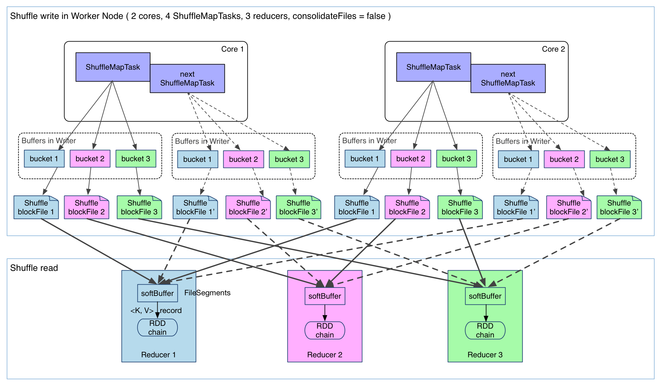
In the diagram there're 4 ShuffleMapTasks to execute in the same worker node with 2 cores. The task result (records of the final RDD in the stage) is written on the local disk (data persistence). Each task has R buffers, R equals the number of reducers (the number if tasks in the next stage). The buffers are called buckets in Spark. By default the size of each bucket is 32KB (100KB before Spark 1.1) and is configurable by spark.shuffle.file.buffer.kb .

In fact bucket is a general concept in Spark that represents the location of the partitioned output of a ShuffleMapTask. Here for simplicity a bucket is referred to an in-memory buffer.

ShuffleMapTask employs the pipelining techinque to compute the result records of the final RDD. Each record is sent to the bucket of its corresponding partition, which is determined by partitioner.partition(record.getKey()). The content of these buckets is written continuously to local disk files called ShuffleBlockFile, or FileSegment for short. Reducers will fetch their FileSegment in shuffle read phase.

An implementation like this is very simple, but has some issues:

1. We may produce too many FileSegment. Each ShuffleMapTask produces R(number of reducers) FileSegment, so M ShuffleMapTask will produce M * R files. For big datasets we could have big M and R, as a result there may be lots of intermediate data files.
2. Buffers could take a lot of space. On a worker node, we could have R * M buckets for each core available to Spark. Spark will reuse the buffer space after a ShuffleMapTask but there could still be R * cores buckets in memory. On a node with 8 cores processing a 1000-reducer job, buckets will take up 256MB (R * cores * 32KB).

Currently, there's no good solution to the second problem. We need to write buffers anyway and if they're too small there will be impact on IO speed. For the first problem, we have a file consolidation solution already implemented in Spark. Let's check it out:

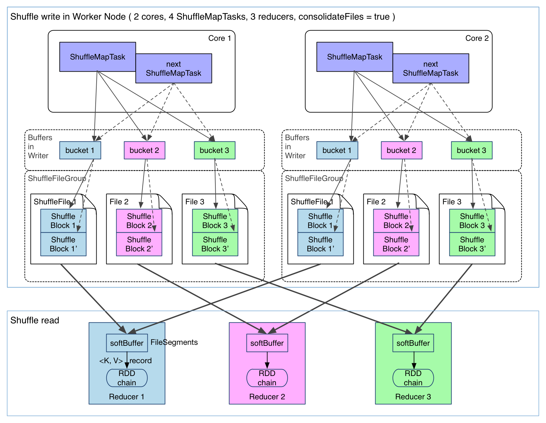
It's clear that from the above diagram, consecutive ShuffleMapTasks running on the same core share a shuffle file. Each task appends its output data, ShuffleBlock i', after the output data of the previous task, ShuffleBlock i. A ShuffleBlock is called a FileSegment. In this way, reducers in the next stage can just fetch the whole file and we reduce the number of files needed in each worker node to cores * R. File consolidation feature can be activated by setting spark.shuffle.consolidateFiles to true.

Shuffle Read

Let's check a physical plan of reduceBykey, which contains ShuffleDependency:

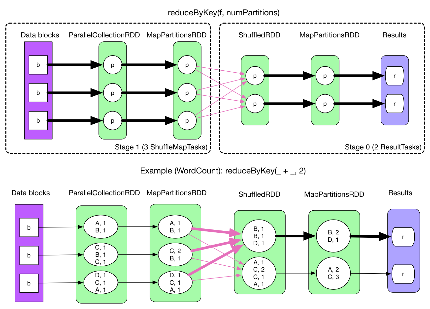
Intuitively, we need to fetch the data of MapPartitionRDD to be able to evaluate ShuffleRDD. Then come the problems:

• When to fetch? Fetch for each ShuffleMapTask or fetch only once after all ShuffleMapTasks are done?
• Fetch and process the records at the same time or fetch and then process?
• Where to store the fetched data?
• How do the tasks of the next stage know the location of the fetched data?

Solutions in Spark:

• When to fetch? Wait after all ShuffleMapTasks end and then fetch. We know that a stage will be executed only after its parent stages are executed, so it's intuitive that the fetch operation begins after all ShuffleMapTasks in the previous stage are done. The fetched FileSegments have to be buffered in memory, so we can't fetch too much before the buffer content is written to disk. Spark limits this buffer size by spark.reducer.maxMbInFlight, here we name it softBuffer. It has default size 48MB. A softBuffer usually contains multiple fetched FileSegments. But sometimes one single segment can fill up the buffer.

• Fetch and process the records at the same time or fetch and then process? Fetch and process the records at the same time. In MapReduce, the shuffle stage fetches the data and then applies combine() logic at the same time. However in MapReduce the reducer input data needs to be sorted, so the reduce() logic is applied after the shuffle-sort process. Since Spark does not require a sorted order for the reducer input data, we don't need to wait until all the data gets fetched to start processing. Then how Spark implements this shuffle and processing? In fact Spark utilizes data structures like HashMap to do the job. Each \<Key, Value> pair from the shuffle process is inserted into a HashMap. If the Key is already present, then the pair is aggregated by func(hashMap.get(Key), Value). In the above WordCount example, the func is hashMap.get(Key) + Value, and its result is updated in the HashMap. This func has a similar role to reduce() in Hadoop, but they differ in details. We illustrate the difference by the following code snippet:

  // MapReduce
  reduce(K key, Iterable<V> values) {
      result = process(key, values)
      return result
  }
  
  // Spark
  reduce(K key, Iterable<V> values) {
      result = null
      for (V value : values)
          result  = func(result, value)
      return result
  }

In Hadoop MapReduce, we can define any data structure we like in process function. It's just a function that takes an Iterable as parameter. We can also choose to cache the values for further processing. In Spark, a foldLeft like technique is used to apply the func. For example, in Hadoop, it's very easy to compute the average out of values: sum(values) / values.length. But it's not the case in the Spark model. We'll come back to this part later.

• Where to store the fetched data? The fetched FileSegments get buffered in softBuffer. Then the data is processed, and written to a configurable location. If spark.shuffle.spill is false, then the write location is only memory. A special data structure, AppendOnlyMap, is used to hold these processed data in memory. Otherwise, the processed data will be written to memory and disk, using ExternalAppendOnlyMap. This data structure can spill the sorted key-value pairs on disk when there isn't enough memory available. A key problem in using both memory and disk is how to find a balance of the two. In Hadoop, by default 70% of the memory is reserved for shuffle data. Once 66% of this part of the memory is used, Hadoop starts the merge-combine-spill process. In Spark a similar strategy is used. We'll talk about its details later in this chapter.

• How do the tasks of the next stage know the location of the fetched data? Recall that in the last chapter, there's an important step: ShuffleMapStage, which will register its final RDD by calling MapOutputTrackerMaster.registerShuffle(shuffleId, rdd.partitions.size). So during the shuffle process, reducers get the data location by querying MapOutputTrackerMaster in the driver process. When a ShuffleMapTask finishes, it will report the location of its FileSegment to MapOutputTrackerMaster.

Now we have discussed the main ideas behind shuffle write and shuffle read as well as some implementation details. Let's dive into some interesting details.

Shuffle Read of Typical Transformations

reduceByKey(func)

We have briefly talked about the fetch and reduce process of reduceByKey(). Note that for an RDD, not all its data is present in the memory at a given time. The processing is always on a record basis. Processed record is rejected if possible. On a record level perspective, the reduce() logic can be shown as below:

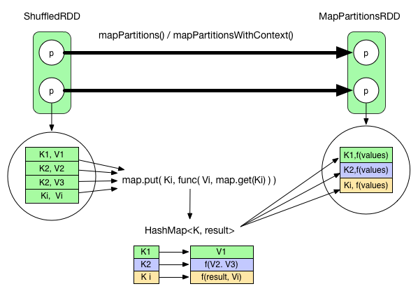
We can see that the fetched records are aggregated using a HashMap, and once all the records are aggregated, we will have the result. The func needs to be commutative.

A mapPartitionsWithContext operation is used to transform the ShuffledRDD to a MapPartitionsRDD.

To reduce network trafic between nodes, we could use map side combine() in Hadoop. It's also feasible in Spark. All we need is to apply the mapPartitionsWithContext in the ShuffleMapStage. For example in reduceByKey , the transformation of ParallelCollectionRDD to MapPartitionsRDD is equivalent to a map side combine.

Comparison between map()->reduce() in Hadoop and reduceByKey in Spark

• map side: there's no difference on the map side. For combine() logic, Hadoop imposes a sort before combine(). Spark applies the combine() logic by using a hash map.
• reduce side: Shuffle process in Hadoop will fetch the data until a certain amount, then applies combine() logic, then merge sort the data to feed the reduce() function. In Spark fetch and reduce is done at the same time (in a hash map), so the reduce function needs to be commutative.

Comparison in terms of memory usage

• map side: Hadoop needs a big, circular buffer to hold and sort the map() output data. But combine() does not need extra space. Spark needs a hash map to do combine(). And persisting records to local disk needs buffers (buckets).
• reduce side: Hadoop needs some memory space to store shuffled data. combine() and reduce() require no extra space since their input is sorted and can be grouped and then aggregated. In Spark, a softBuffer is needed for fetching. A hash map is used for storing the result of combine() and reduce(), if only memory is used in processing data. However, part of the data can be stored on disk if configured to use both memory and disk.

groupByKey(numPartitions)

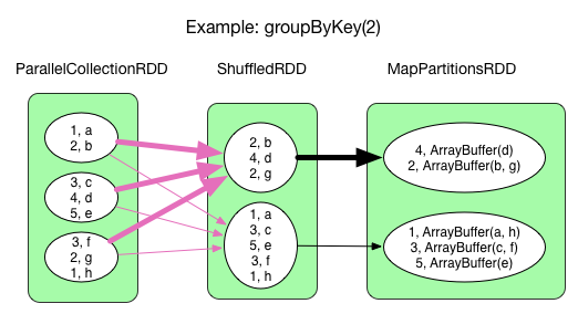
The process is similar to that of reduceByKey(). The func becomes result = result ++ record.value. This means that each key's values are grouped together without further aggregation.

distinct(numPartitions)

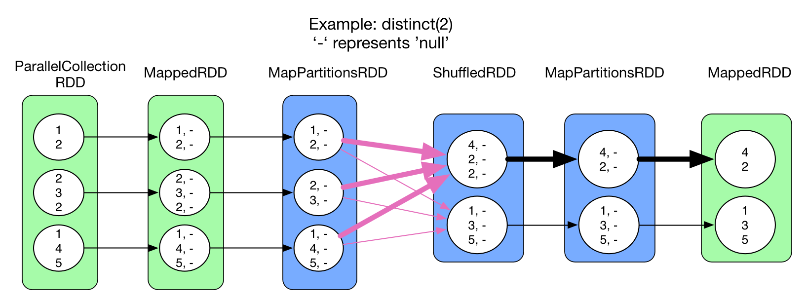
Similar to reduceByKey(). The func is result = result == null ? record.value : result. This means that we check the existence of the record in the HashMap. If it exists, reject the record, otherwise insert it into the map. Like reduceByKey(), there's map side combine().

cogroup(otherRDD, numPartitions)

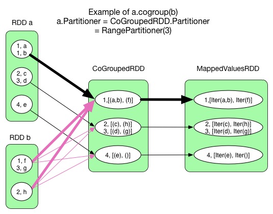
There could be 0, 1 or multiple ShuffleDependency for a CoGroupedRDD. But in the shuffle process we don't create a hash map for each shuffle dependency, but one hash map for all of them. Different from reduceByKey, the hash map is constructed in RDD's compute() rather than in mapPartitionsWithContext().

A task of this RDD's execution will allocate an Array[ArrayBuffer]. This array contains the same number of empty ArrayBuffers as the number of input RDDs. So in the example we have 2 ArrayBuffers in each task. When a key-value pair comes from RDD A, we add it to the first ArrayBuffer. If a key-value pair comes from RDD B, then it goes to the second ArrayBuffer. Finally a mapValues() operation transforms the values into the correct type: (ArrayBuffer, ArrayBuffer) => (Iterable[V], Iterable[W]).

intersection(otherRDD) and join(otherRDD, numPartitions)

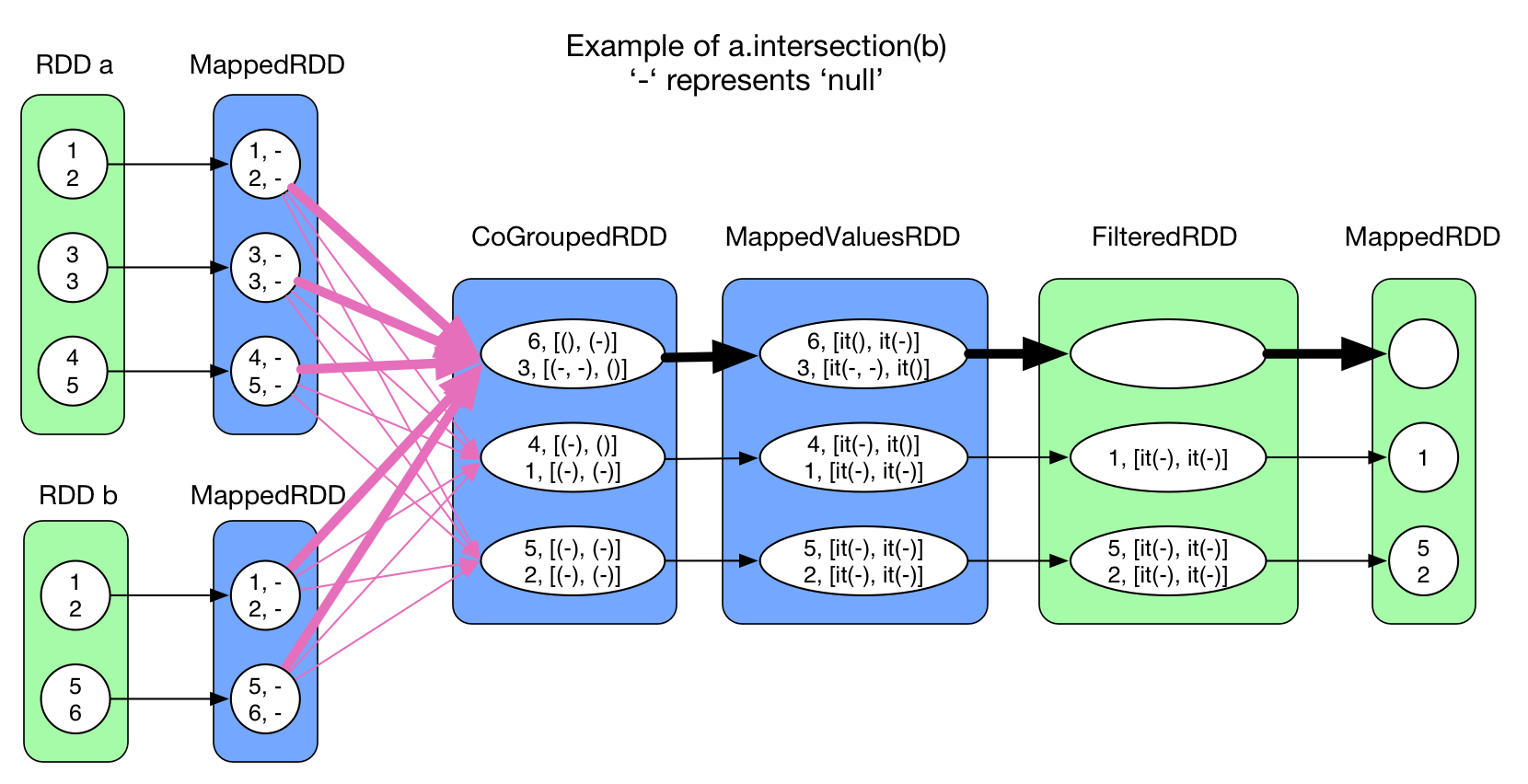
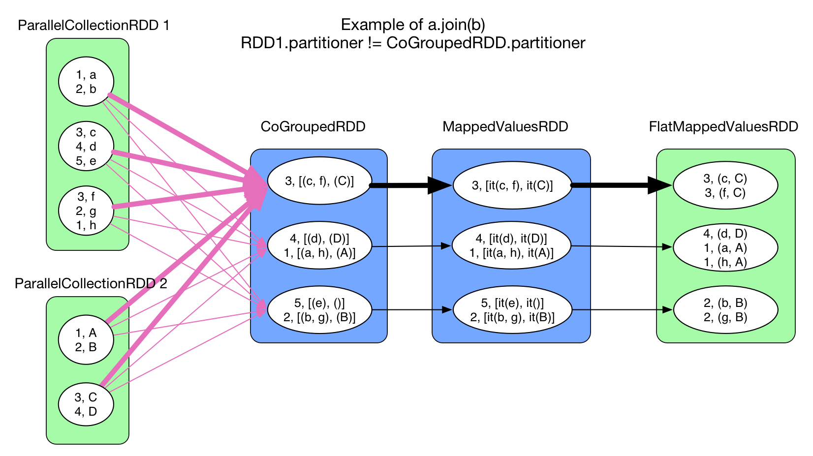
This two operations both use cogroup, so their shuffle process is identical to cogroup.

sortByKey(ascending, numPartition)

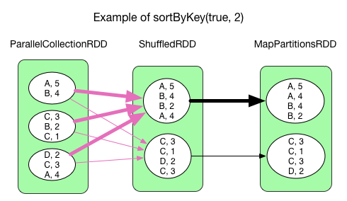
The processing logic of sortByKey() is a little different from reduceByKey() as it does not use a HashMap to handle incoming fetched records. Instead, all key-value pairs are range partitioned. The records of the same partition is sorted by key.

coalesce(numPartitions, shuffle = true)

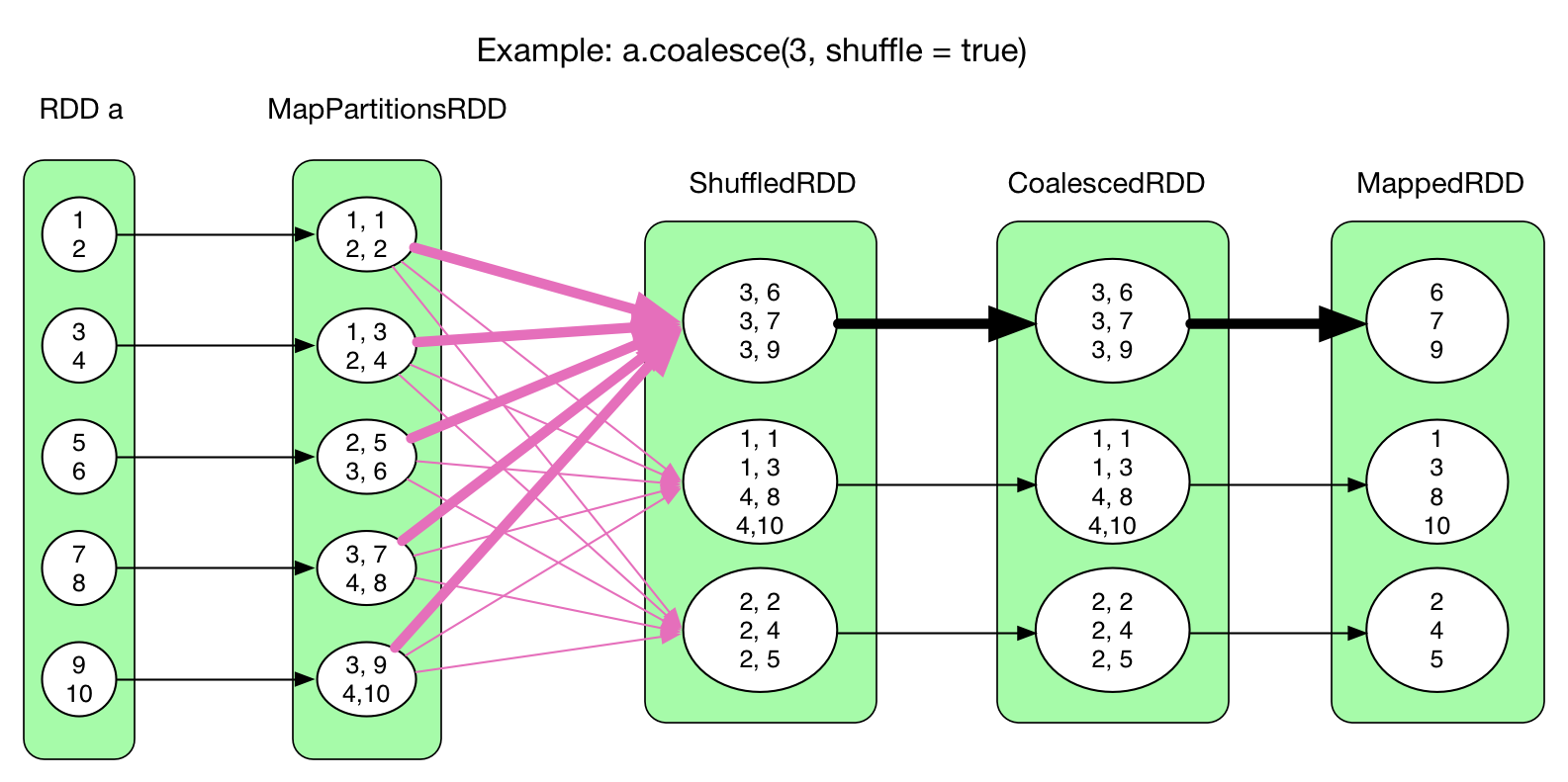
coalesce() would create a ShuffleDependency, but it actually does not need to aggregate the fetched records, so no hash map is needed.

HashMap in Shuffle Read

So as we have seen, hash map is a frequently used data structure in Spark's shuffle process. Spark has 2 versions of specialized hash map: in memory AppendOnlyMap and memory-disk hybrid ExternalAppendOnlyMap. Let's look at some details of these two hash map implementations.

AppendOnlyMap

The Spark documentation describes AppendOnlyMap as "A simple open hash table optimized for the append-only use case, where keys are never removed, but the value for each key may be changed". Its implementation is simple: allocate a big array of Object, as the following diagram shows. Keys are stored in the blue sections, and values are in the white sections.

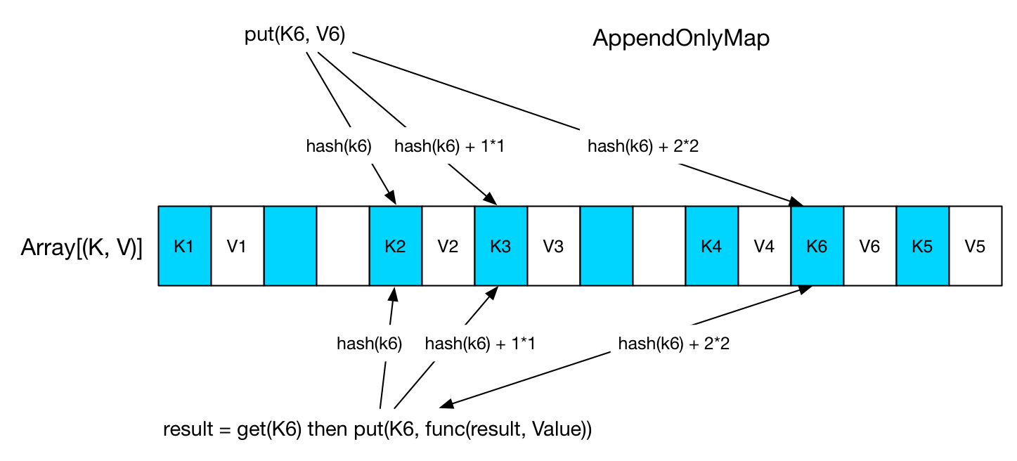
When a put(K, V) is issued, we locate the slot in the array by hash(K). If the position is already occupied, then quadratic probing technique is used to find the next slot.. For the example in the diagram, K6, a third probing has found an empty slot after K4, then the value is inserted after the key. When get(K6), we use the same technique to find the slot, get V6 from the next slot, compute a new value, then write it to the position of V6.

Iteration over the AppendOnlyMap is just a scan of the array.

If 70% of the allocated array is used, then it will grow twice as large. Keys will be rehashed and the positions re-organized.

There's a destructiveSortedIterator(): Iterator[(K, V)] method in AppendOnlyMap. It returns sorted key-value pairs. It's implemented like this: first compact all key-value pairs to the front of the array and make each key-value pair in a single slot. Then Array.sort() is called to sort the array. As its name indicates, this operation will destroy the structure.

ExternalAppendOnlyMap

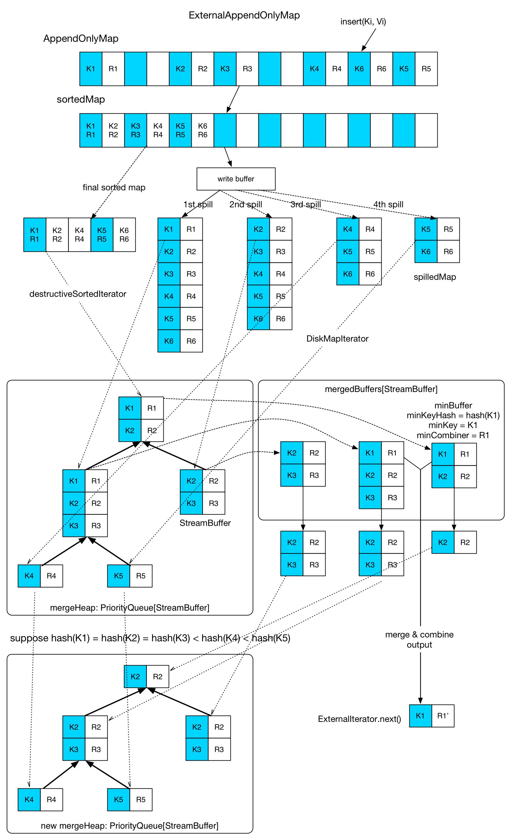
Compared with AppendOnlyMap, the implementation of ExternalAppendOnlyMap is more sophisticated. Its concept is similar to the shuffle-merge-combine-sort process in Hadoop.

ExternalAppendOnlyMap holds an AppendOnlyMap. Incoming key-value pairs are inserted into the AppendOnlyMap. When AppendOnlyMap is about to grow its size, we'll check the available memory space. If there's still enough space, the AppendOnlyMap doubles its size, otherwise all its key-value pairs are sorted and then spilled onto local disk (by using destructiveSortedIterator()). In the diagram, there're 4 spills of this map. In each spill, a spillMap file will be generated and a new, empty AppendOnlyMap will be instantiated to receive incoming key-value pairs. In ExternalAppendOnlyMap, when a key-value pair is inserted, it gets aggregated only with the in memory part (the AppendOnlyMap). So it means when asked for the final result, a global merge-aggregate needs to be performed on all spilled maps and the in memory AppendOnlyMap.

Global merge-aggregate runs as follows. Firstly the in memory part (AppendOnlyMap) is sorted to a sortedMap. Then DestructiveSortedIterator (for sortedMap) or DiskMapIterator (for on disk spillMap) will be used to read a part of the key-value pairs into a StreamBuffer. Then the StreamBuffer is inserted into a mergeHeap. In each StreamBuffer, all records have the same hash(key). Suppose that in the example, we have hash(K1) == hash(K2) == hash(K3) < hash(K4) < hash(K5). As a result, the first 3 records of the first spilled map are read into the same StreamBuffer. The merge is simple: get StreamBuffers with the same key hash using a heap, then put them into an ArrayBuffer[StreamBuffer](mergedBuffers) for merge. The first inserted StreamBuffer is called minBuffer, the key of its first key-value pair is minKey. One merge operation will aggregate all KV pairs with minKey in the mergedBuffer and then output the result. When a merge operation in mergedBuffer is over, remaining KV pairs will return to the mergeHeap, and empty StreamBuffer will be replaced by a new read from in-memory map or on-disk spill.

There're still 3 points needed to be discussed:

• Available memory check. Hadoop allocates 70% of the memory space of a reducer for shuffle-sort. Similarly, Spark has spark.shuffle.memoryFraction * spark.shuffle.safetyFraction (defaults to 0.3 * 0.8) for ExternalAppendOnlyMap. It seems that Spark is more conservative. Moreover, this 24% of memory space is shared by all reducers in the same executor. An executor holds a ShuffleMemoryMap: HashMap[threadId, occupiedMemory] to monitor memory usage of all ExternalAppendOnlyMaps in each reducer. Before an AppendOnlyMap grows, the total memory usage after the growth will be computed using the information in ShuffleMemoryrMap, to see if there's enough space. Also notice that the first 1000 records will not trigger the spill check.

• AppendOnlyMap size estimation. To know the size of an AppendOnlyMap, we can compute the size of every object referenced in the structure during each growth. But this takes too much time. Spark has an estimation algorithm with O(1) complexity. Its core concept is to see how the map size changes after the insertion and aggregation of a certain amount of records to estimate the structure size. Details are in SizeTrackingAppendOnlyMap and SizeEstimator.

• Spill process. Like the shuffle write, Spark creates a buffer when spilling records to disk. Its size is spark.shuffle.file.buffer.kb, defaulting to 32KB. Since the serializer also allocates buffers to do its job, there'll be problems when we try to spill lots of records at the same time. Spark limits the records number that can be spilled at the same time to spark.shuffle.spill.batchSize, with a default value of 10000.

Discussion

As we've seen in this chapter, Spark is way more flexible in the shuffle process compared to Hadoop's fixed shuffle-combine-merge-reduce model. It's possible in Spark to combine different shuffle strategies with different data structures to design an appropriate shuffle process based on the semantic of the actual transformation.

So far we've discussed the shuffle process in Spark without sorting as well as how this process gets integrated into the actual execution of the RDD chain. We've also talked about memory and disk issues and compared some details with Hadoop. In the next chapter we'll try to describe job execution from an inter-process communication perspective. The shuffle data location problem will also be mentioned.

Plus to this chapter, thers's the outstanding blog (in Chinese) by Jerry Shao, Deep Dive into Spark's shuffle implementation.