Spark Logical Plan

An example of general logical plan

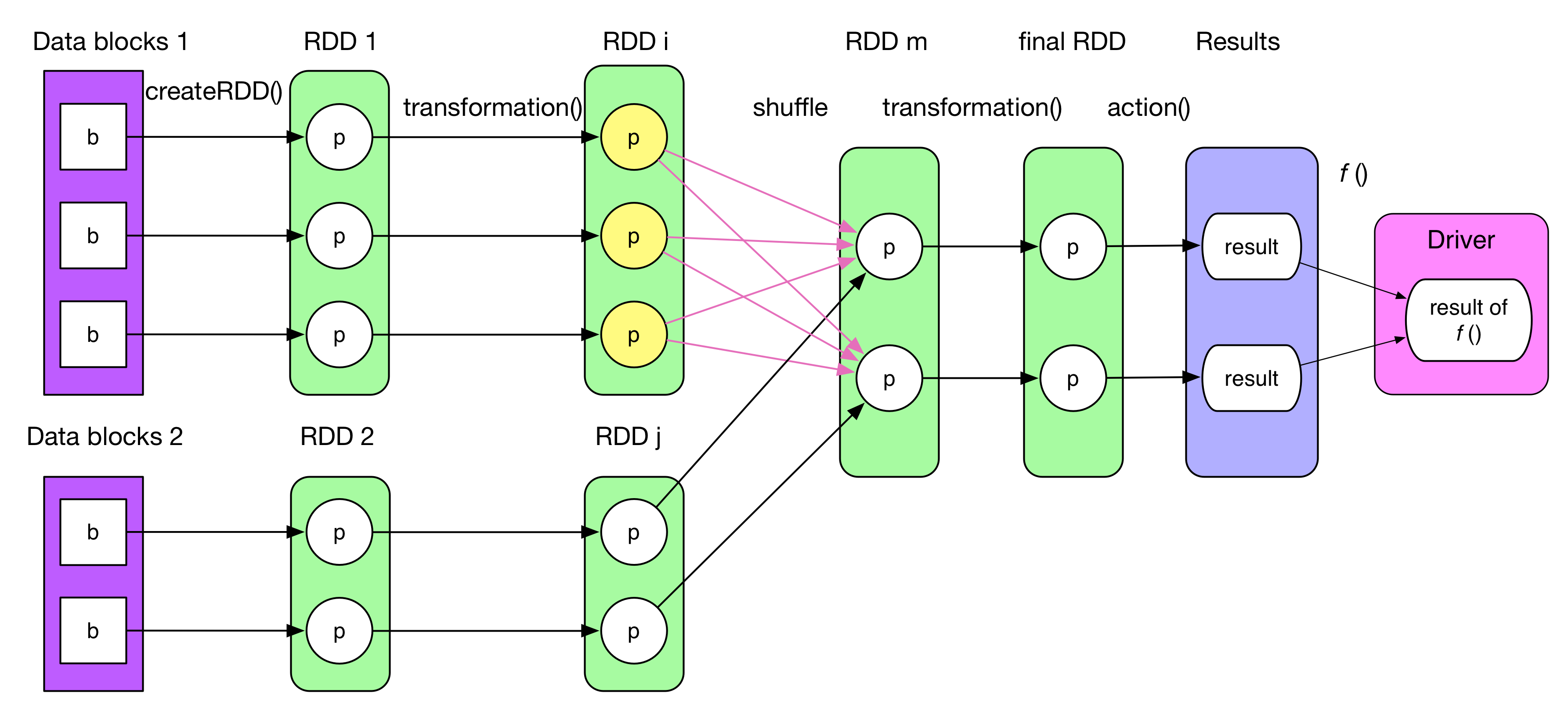
The picture above illustrates a general job logical plan which takes 4 steps to get the final result:

1. Construct the initial RDD from any source.(in-memory data, local file, HDFS, HBase, etc). (Note that parallelize() is equivalent to createRDD() mentioned in the previous chapter)

2. A series of transformation operations on RDD, denoted as transformation(), each transformation() produces one or more RDD[T]s, where T can be any type in Scala.

   Need to mention that, for key-value pair `RDD[(K, V)]`, it will be handy if `K` is a basic type, like `Int`, `Double`, `String`, etc. It can not be collection type, like `Array`, `List`, etc, since it is hard to define `partition` function on collections

3. Action operation, denoted as action() is called on final RDD, then each partition produces a result

4. These results will be sent to the driver, then f(List[Result]) will be computed as the final result to client side, for example, count() takes two steps, action() and sum().

RDD can be cached into memory or on hard disk, by calling cache(), persist() or checkpoint(). The number of partitions is usually set by user. Partition relationship between 2 RDDs can be not 1 to 1. In the picture above, we can see not only 1 to 1 relationship, but also many to many ones.

Logical Plan

When writing your spark code, you might also have a dependency diagram in you mind (like the one above). However, the reality is that some more RDDs will be produced.

In order to make this more clear, we will talk about :

• How to produce RDD ? What kind of RDD should be produced ?
• How to build dependency relationship between RDDs ?

1. How to produce RDD? What RDD should be produced?

A transformation() usually returns a new RDD, but some transformation()s which are more complicated and contain several sub-transformation() produce multiple RDDs. That's why the number of RDDs is, in fact, more than we thought.

Logical plan is essentially a computing chain. Every RDD has a compute() method which takes the input records of the previous RDD or data source, then performs transformation(), finally outputs computed records.

What RDD to be produced depends on the computing logic. Let's talk about some typical transformation() and the RDDs they produce.

We can learn about the meaning of each transformation() on Spark site. More details are listed in the following table, where iterator(split) means for each record in partition. There are some blanks in the table, because they are complex transformation() producing multiple RDDs, they will be illustrated soon after.

Transformation	Generated RDDs	Compute()
map(func)	MappedRDD	iterator(split).map(f)
filter(func)	FilteredRDD	iterator(split).filter(f)
flatMap(func)	FlatMappedRDD	iterator(split).flatMap(f)
mapPartitions(func)	MapPartitionsRDD	f(iterator(split))
mapPartitionsWithIndex(func)	MapPartitionsRDD	f(split.index, iterator(split))
sample(withReplacement, fraction, seed)	PartitionwiseSampledRDD	PoissonSampler.sample(iterator(split)) BernoulliSampler.sample(iterator(split))
pipe(command, [envVars])	PipedRDD
union(otherDataset)
intersection(otherDataset)
distinct([numTasks]))
groupByKey([numTasks])
reduceByKey(func, [numTasks])
sortByKey([ascending], [numTasks])
join(otherDataset, [numTasks])
cogroup(otherDataset, [numTasks])
cartesian(otherDataset)
coalesce(numPartitions)
repartition(numPartitions)

2. How to build RDD relationship?

We need to figure out the following things:

• RDD dependencies. RDD x depends on one parent RDD or several parent RDDs?
• How many partitions are there in RDD x?
• What's the relationship between the partitions of RDD x and those of its parent RDD(s)? One partition depends one or several partition of parent RDD?

The first question is trivial, such as x = rdda.transformation(rddb), e.g., val x = a.join(b) means that RDD x depends both RDD a and RDD b

For the second question, as mentioned before, the number of partitions is defined by user, by default, it takes max(numPartitions[parent RDD 1], ..., numPartitions[parent RDD n])

The third one is a little bit complex, we need to consider the meaning of a transformation(). Different transformation()s have different dependency. For example, map() is 1:1, while groupByKey() produces a ShuffledRDD in which each partition depends on all partitions in its parent RDD. Besides this, some transformation() can be more complex.

In spark, there are 2 kinds of dependencies which are defined in terms of parent RDD's partition:

• NarrowDependency (OneToOneDependency, RangeDependency)

  each partition of the child RDD depends on a small number of partitions of the parent RDD, i.e. a child partition depends the **entire** parent partition. (**full dependency**)

• ShuffleDependency (or wide dependency, mentioned in Matei's paper)

  multiple child partitions depends on a parent partition, i.e. each child partition depends **a part of** the parent partition. (**partial dependency**)

For example, map leads to a narrow dependency, while join leads to to wide dependencies (unless the two parents are hash-partitioned).

On the other hand, each child partition can depend on one partition in parent RDD, or some partitions in parent RDD.

Note that:

• For NarrowDependency, whether a child partition needs one or multiple parent partition depends on getParents(partition i) function in child RDD. (More details later)
• ShuffleDependency is like shuffle dependency in MapReduce（mapper partitions its output, then each reducer will fetch all the needed output partitions via http.fetch)

The two dependencies are illustrated in the following picture.

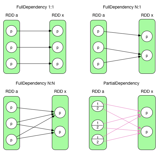
According to the definition, the two on the first row are NarrowDependency and the last one is ShuffleDependency.

Need to mention that the left one on the second row is a very rare case between two RDD. It is a NarrowDependency (N:N) whose logical plan is like ShuffleDependency, but it is a full dependency. It can be created by some tricks. We will not talk about this, because, more strictly, NarrowDependency essentially means each partition of the parent RDD is used by at most one partition of the child RDD. Some typical RDD dependencies will be talked about soon.

To conclude, partition dependencies are listed as below

• NarrowDependency (black arrow)
  • RangeDependency -> only for UnionRDD
  • OneToOneDependency (1:1) -> e.g. map, filter
  • NarrowDependency (N:1) -> e.g. join co-partitioned
  • NarrowDependency (N:N) -> rare case
• ShuffleDependency (red arrow)

Note that, in the rest of this chapter, NarrowDependency will be represented by black arrow and ShuffleDependency are red ones.

NarrowDependency and ShuffleDependency are needed for physical plan which will be talked about in the next chapter.

How to compute records in RDD x

An OneToOneDependency case is shown in the picture below. Although it is a 1 to 1 relationship between two partitions, it doesn't mean that records are read and computed one by one.

The difference between the two patterns on the right side is similar to the following code snippets.

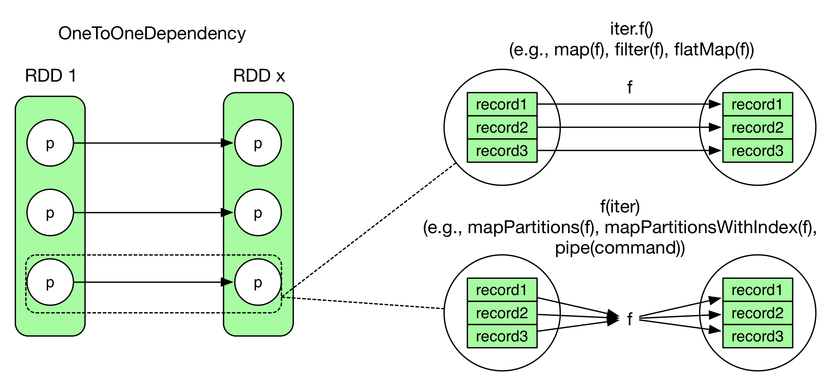
code1 of iter.f()

int[] array = {1, 2, 3, 4, 5}
for(int i = 0; i < array.length; i++)
    f(array[i])

code2 of f(iter)

int[] array = {1, 2, 3, 4, 5}
f(array)

3. Illustration of typical dependencies and their computation

1) union(otherRDD)

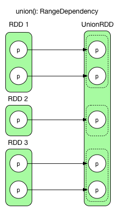
union() simply combines two RDDs together. It never changes data of a partition. RangeDependency(1:1) retains the borders of original RDDs in order to make it easy to revisit the partitions from RDD produced by union()

2) groupByKey(numPartitions) [changed in 1.3]

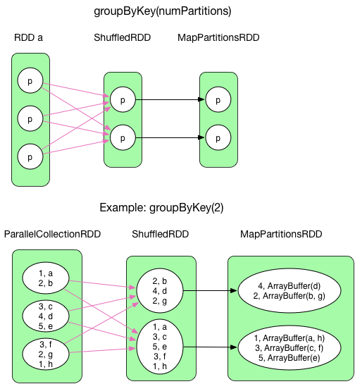
We have talked about groupByKey's dependency before, now we make it more clear.

groupByKey() combines records with the same key by shuffle. The compute() function in ShuffledRDD fetches necessary data for its partitions, then take mapPartition() operation (like OneToOneDependency), MapPartitionsRDD will be produced by aggregate(). Finally, ArrayBuffer type in the value is casted to Iterable

`groupByKey()` has no map side combine, because map side combine does not reduce the amount of data shuffled and requires all map side data be inserted into a hash table, leading to more objects in the old gen.

`ArrayBuffer` is essentially `a CompactBuffer` which is an append-only buffer similar to ArrayBuffer, but more memory-efficient for small buffers.

2) reduceyByKey(func, numPartitions) [changed in 1.3]

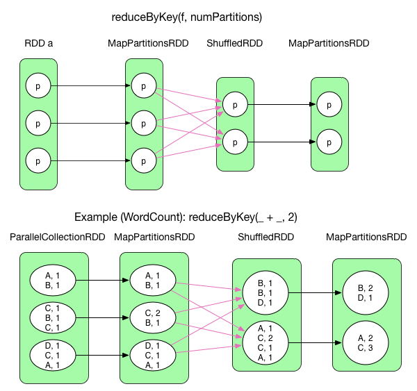
reduceByKey() is similar to MapReduce. The data flow is equivalent. redcuceByKey enables map side combine by default, which is carried out by mapPartitions before shuffle and results in MapPartitionsRDD. After shuffle, aggregate + mapPartitions is applied to ShuffledRDD. Again, we get a MapPartitionsRDD

3) distinct(numPartitions)

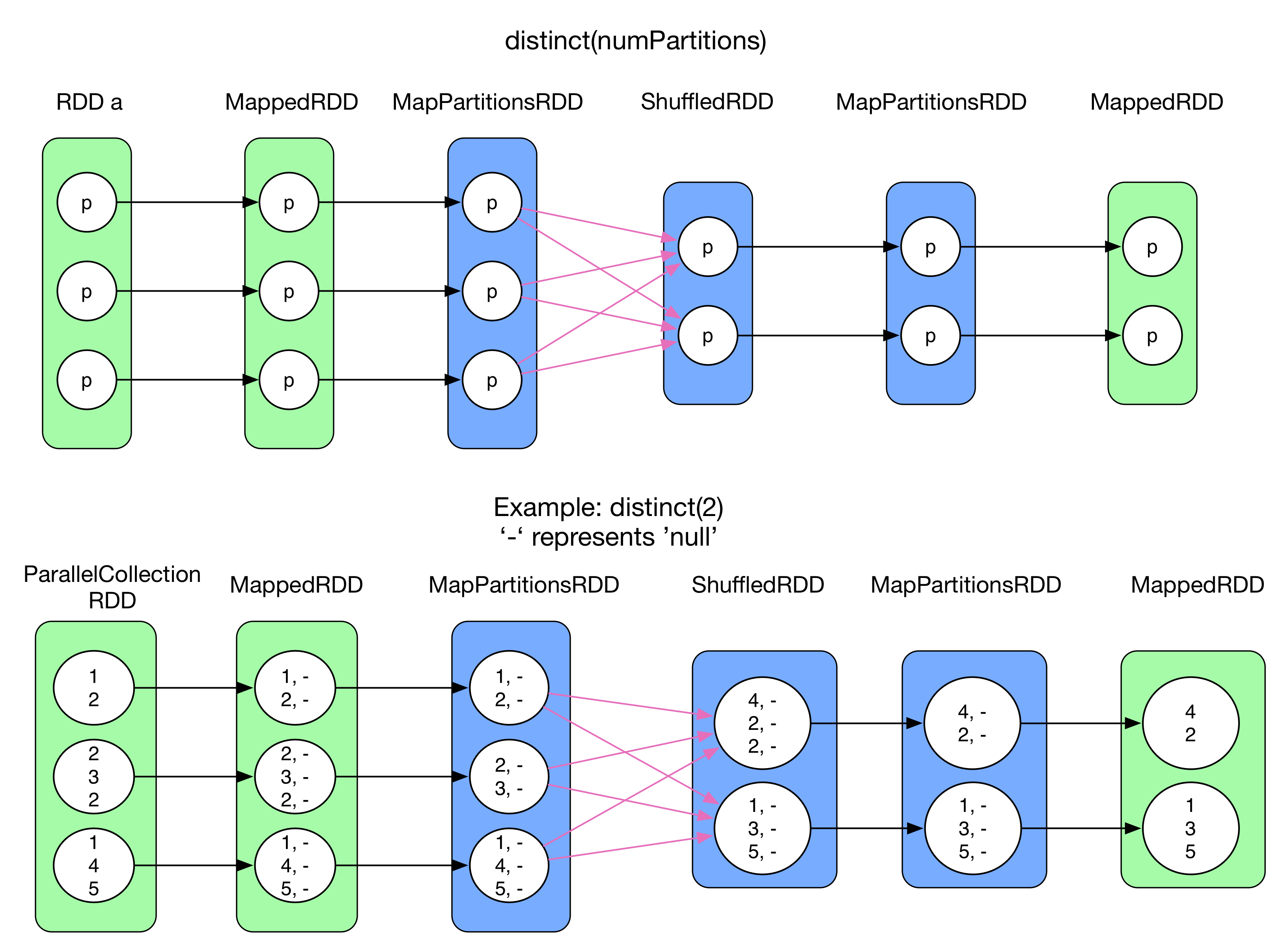
distinct() aims to deduplicate RDD records. Since duplicated records can be found in different partitions, shuffle is needed to deduplicate records by using aggregate(). However, shuffle need RDD[(K, V)]. If the original records have only keys, e.g. RDD[Int], then it should be completed as <K, null> by map() (MappedRDD). After that, reduceByKey() is used to do some shuffle (mapSideCombine->reduce->MapPartitionsRDD). Finally, only key is taken from <K, null> by map()(MappedRDD). ReduceByKey() RDDs are colored in blue

4) cogroup(otherRDD, numPartitions)

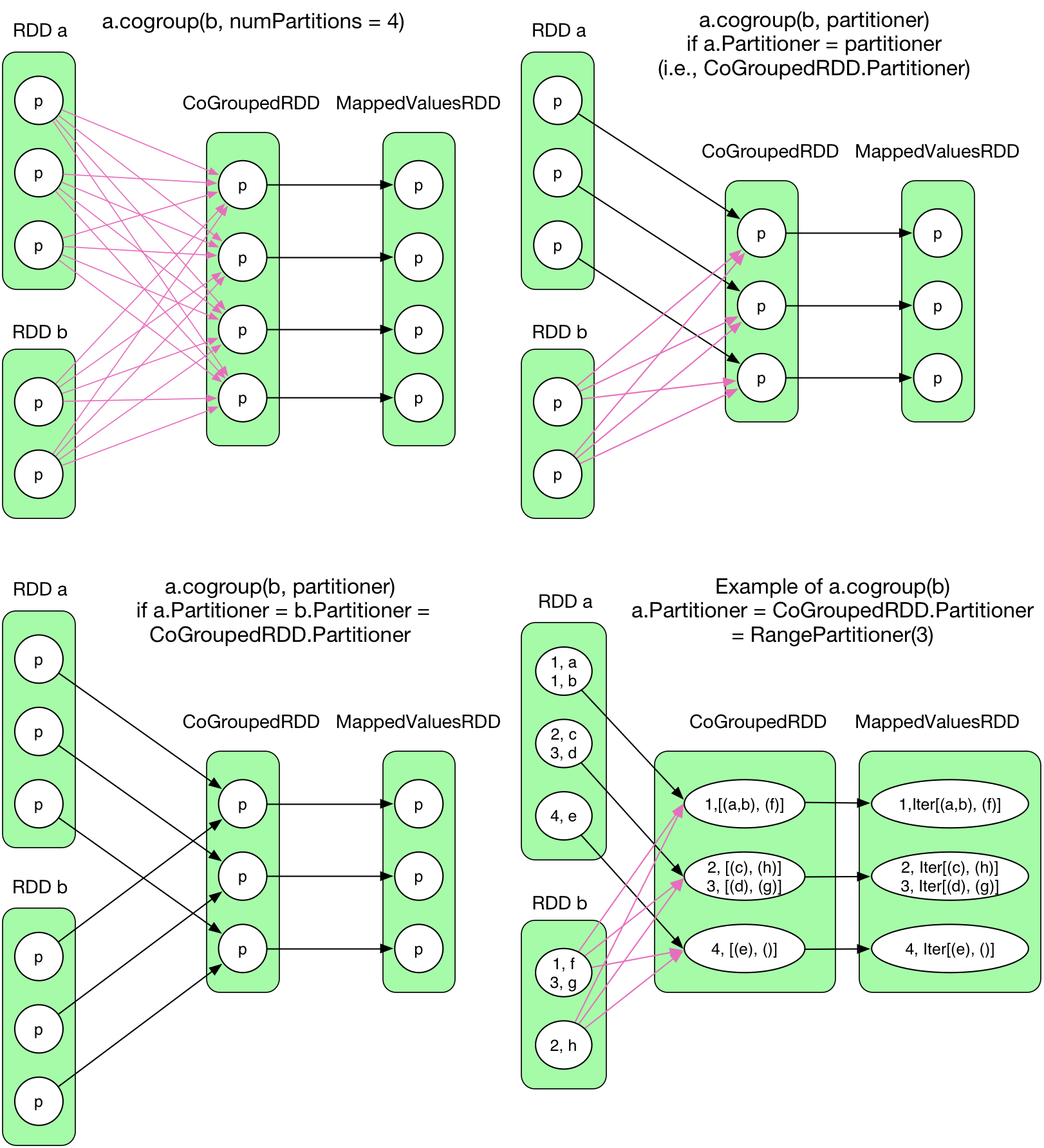
Different from groupByKey(), cogroup() aggregates 2 or more RDDs. What's the relationship between GoGroupedRDD and (RDD a, RDD b)? ShuffleDependency or OneToOneDependency？

• number of partition

  The # of partition in CoGroupedRDD is defined by user, it has nothing to do with RDD a and RDD b. However, if #partition of CoGroupedRDD is different from the one of RDD a/b, then it is not an OneToOneDependency.

• type of partitioner

  The partitioner defined by user (HashPartitioner by default) for cogroup() decides where to put the its results. Even if RDD a/b and CoGroupedRDD have the same # of partition, while their partitioner are different, it can not be OneToOneDependency. Let's take the examples in the picture above, RDD a is RangePartitioner, RDD b is HashPartitioner, and CoGroupedRDD is RangePartitioner with the same # partition as RDD a. Obviously, the records in each partition of RDD a can be directly sent to the corresponding partitions in CoGroupedRDD, but those in RDD b need to be divided in order to be shuffled into the right partitions of CoGroupedRDD.

To conclude, OneToOneDependency occurs iff the partitioner type and #partitions of 2 RDDs and CoGroupedRDD are the same, otherwise, the dependency must be a ShuffleDependency. More details can be found in CoGroupedRDD.getDependencies()'s source code

How does spark deal with the fact that CoGroupedRDD's partition depends on multiple parent partitions?

Firstly, CoGroupedRDD put all needed RDD into rdds: Array[RDD]

Then,

Foreach rdd = rdds(i):
    if CoGroupedRDD and rdds(i) are OneToOneDependency
        Dependecy[i] = new OneToOneDependency(rdd)
    else
        Dependecy[i] = new ShuffleDependency(rdd)

Finally, it returns deps: Array[Dependency] which is an array of Dependency corresponding to each parent RDD.

Dependency.getParents(partition id) returns partitions: List[Int] which are the necessary parent partitions of the specified partition (partition id) with respect to the given Dependency

getPartitions() tells how many partitions are in RDD and how each partition is serialized.

5) intersection(otherRDD)

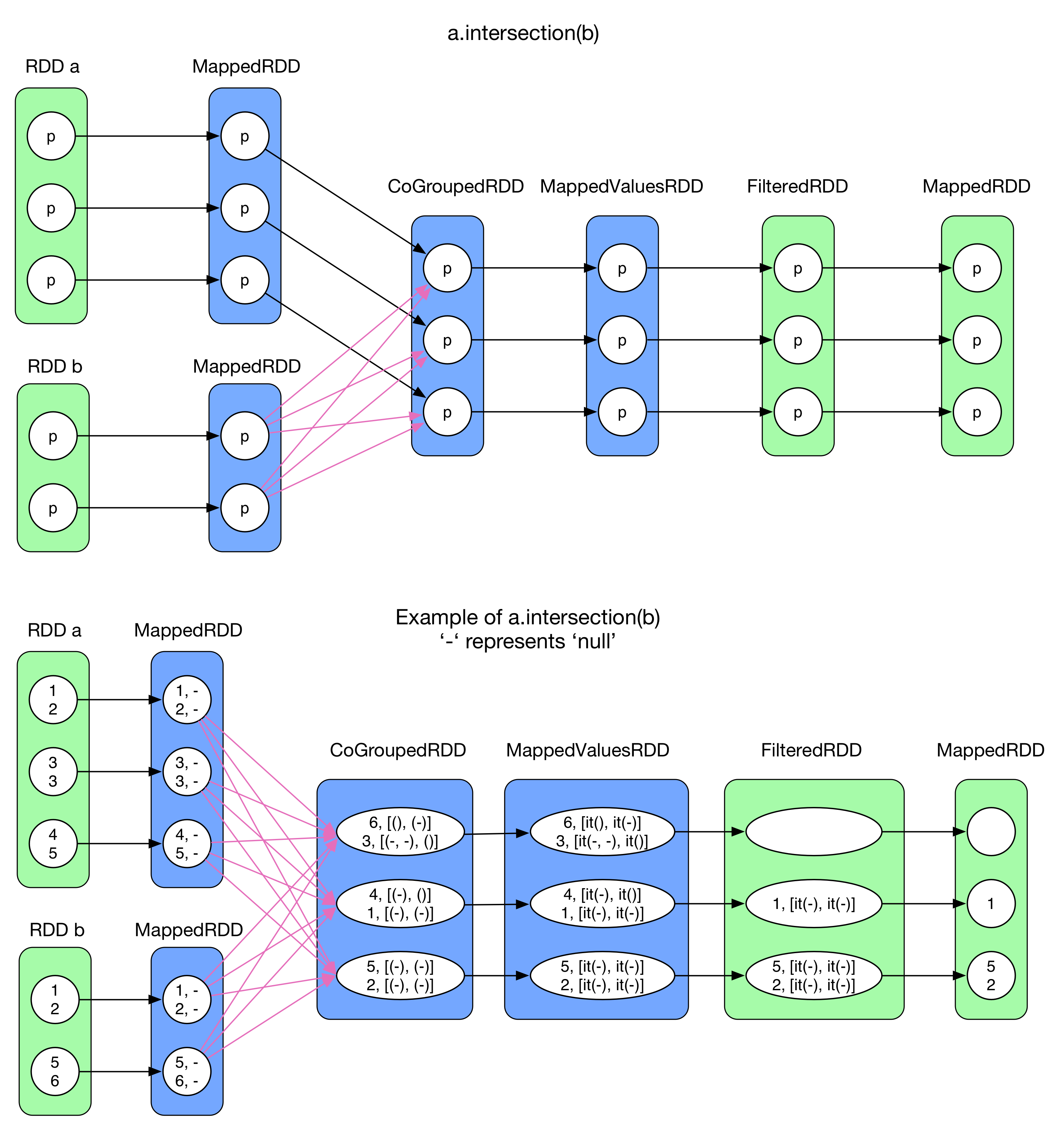
intersection() aims to extract all the common elements from RDD a and b. RDD[T] is mapped into RDD[(T, null)], where T can not be any collections, then a.cogroup(b) (colored in blue). filter() only keeps records where neither of [iter(groupA()), iter(groupB())] is empty (FilteredRDD). Finally, only keys() are kept (MappedRDD)

6) join(otherRDD, numPartitions)

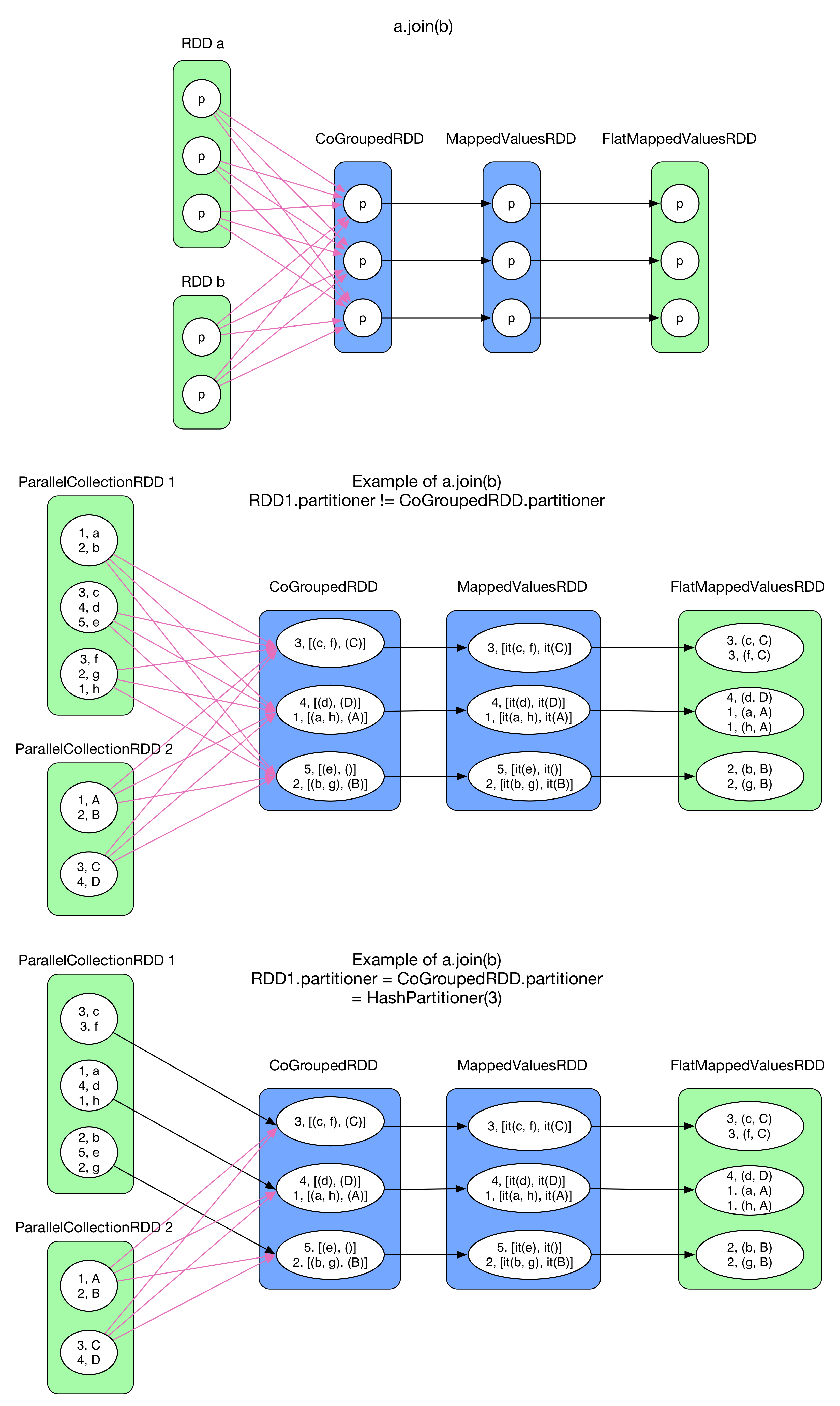
join() takes two RDD[(K, V)], like join in SQL. Similar to intersection(), it does cogroup() first and results in a MappedValuesRDD whose type is RDD[(K, (Iterable[V1], Iterable[V2]))], then compute the Cartesian product between the two Iterable, finally flatMap() is called.

Here are two examples, in the first one, RDD 1 and RDD 2 use RangePartitioner, CoGroupedRDD takes HashPartitioner which is different from RDD 1/2, so it's a ShuffleDependency. In the second one, RDD 1 is initially partitioned on key by HashPartitioner and gets 3 partition which is the same as the one CoGroupedRDD takes, so it's a OneToOneDependency. Furthermore, if RDD 2 is also initially divided by HashPartitioner(3), then there is no ShuffleDependency. This kind of join is called hashjoin()

7) sortByKey(ascending, numPartitions)

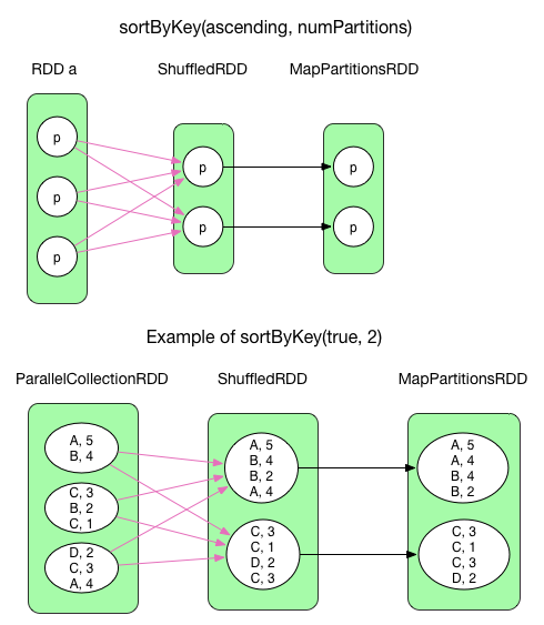
sortByKey() sorts records of RDD[(K, V)] by key. ascending is a self-explanatory boolean flag. It produces a ShuffledRDD which takes a rangePartitioner. The partitioner decides the border of each partition, e.g. the first partition takes records with keys from char A to char B, and the second takes those from char C to char D. Inside each partition, records are sorted by key. Finally, the records in MapPartitionsRDD are in order.

sortByKey() use Array to store records of each partition, then sorts them.

8) cartesian(otherRDD)

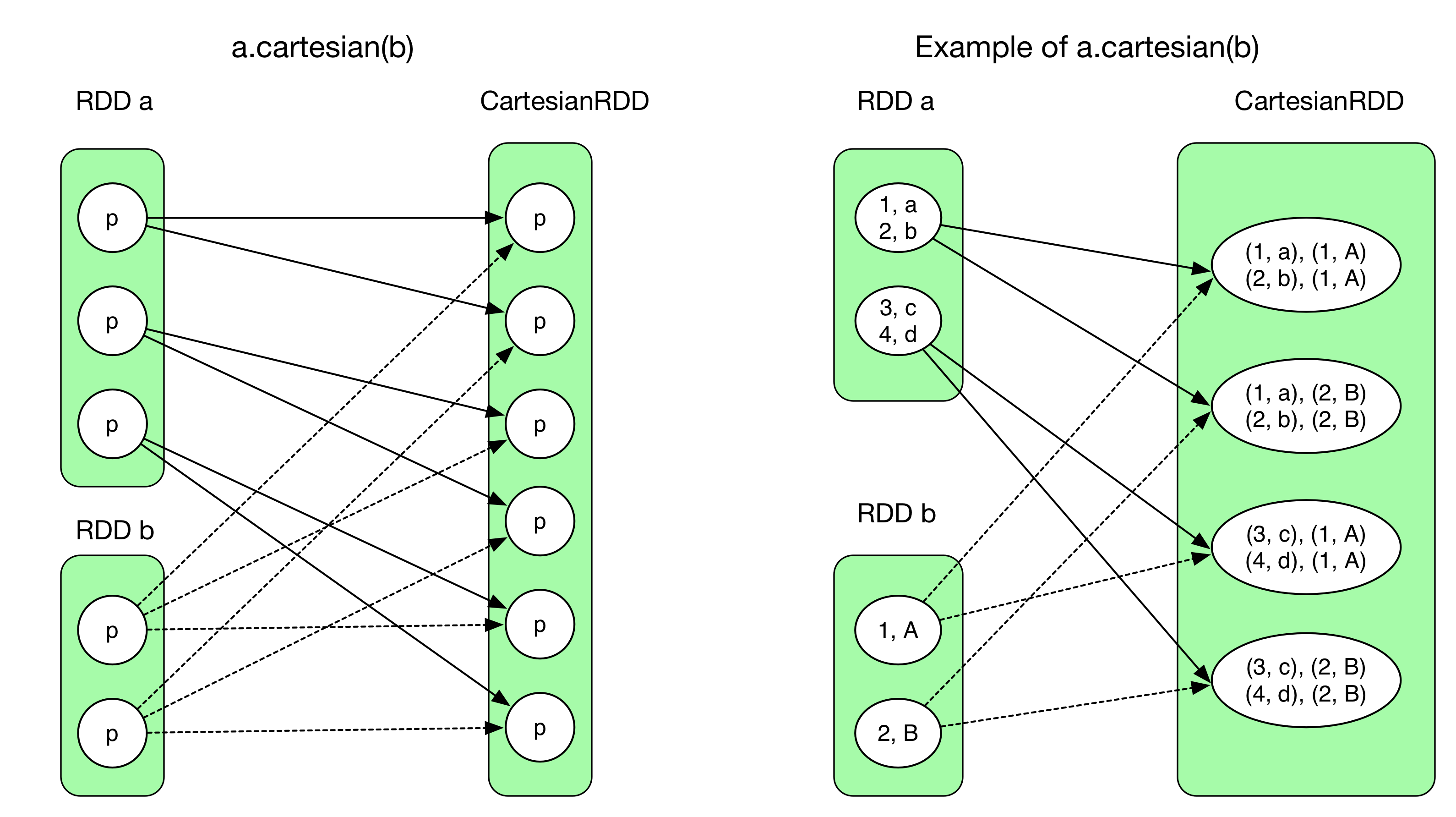
Cartesian() returns a Cartesian product of 2 RDDs. The resulting RDD has #partition(RDD a) x #partition(RDD b) partitions.

Need to pay attention to the dependency, each partition in CartesianRDD depends 2 entire parent RDDs. They are all NarrowDependency.

CartesianRDD.getDependencies() returns rdds: Array(RDD a, RDD b). The ith partition of CartesianRDD depends:

• a.partitions(i / #partitionA)
• b.partitions(i % #partitionB)

9) coalesce(numPartitions, shuffle = false)

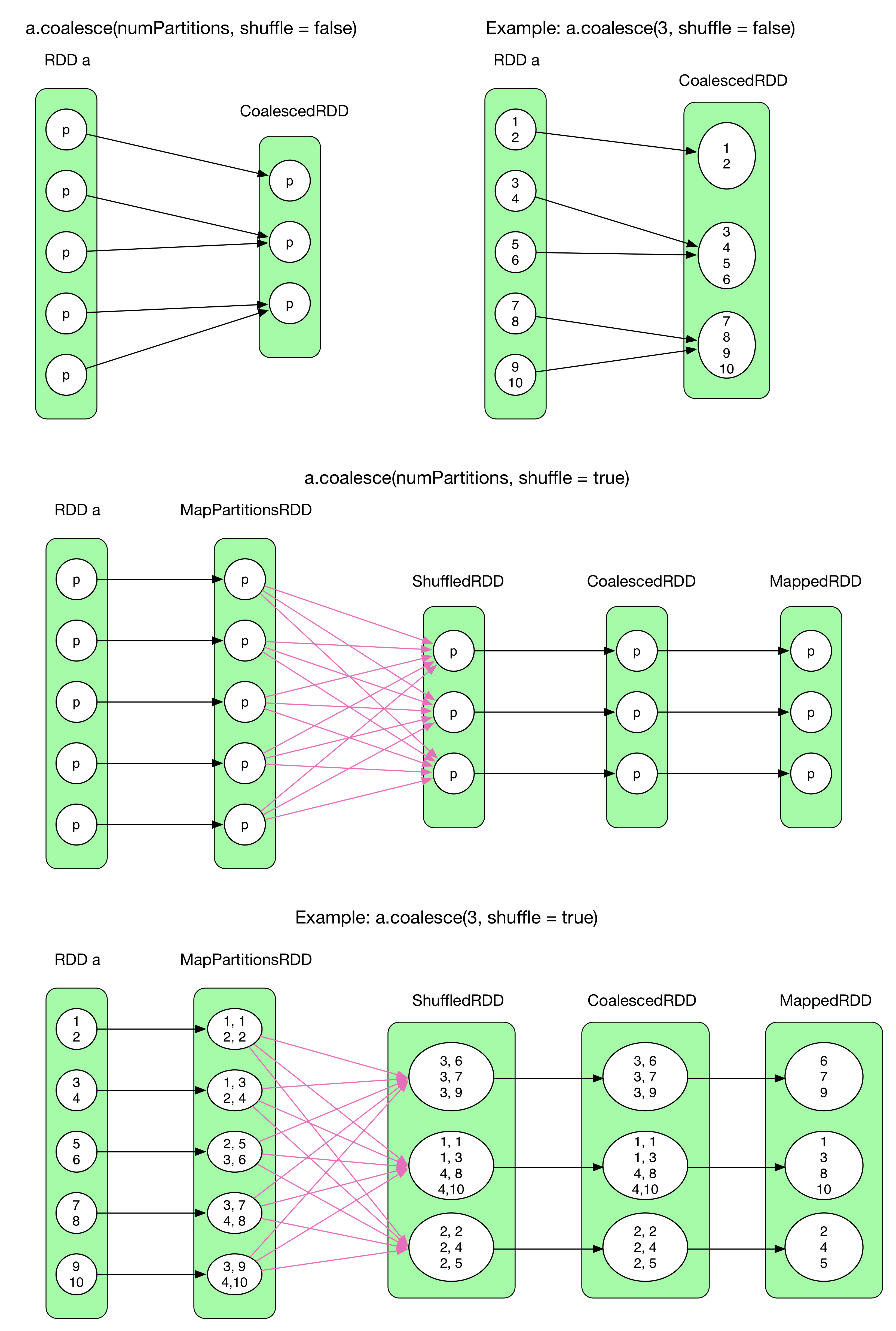
coalesce() can reorganize partitions, e.g. decrease # of partitions from 5 to 3, or increase from 5 to 10. Need to notice that when shuffle = false, we can not increase partitions, because that will force a shuffle while we don't want shuffle, which is nonsense.

To understand coalesce(), we need to know the relationship between CoalescedRDD's partitions and its parent partitions

• coalesce(shuffle = false) As shuffle is disabled, what we need to do is just to group certain parent partitions. In fact, there are many factors to take into consideration, e.g. # records in partition, locality ,balance, etc. Spark has a rather complicated algorithm to do with that. (we will not talk about that for the moment). For example, a.coalesce(3, shuffle = false) is essentially a NarrowDependency of N:1.

• `coalesce(shuffle = true)`

  When shuffle is enabled, coalesce simply divides all records of RDD in N parts, which can be done by the following trick (like round-robin algorithm):

  • for each partition, every record is assigned a key which is an increasing number.
  • hash(key) leads to a uniform records distribution on all different partitions.

  In the second example, every element in RDD a is combined with a increasing key (on the left side of the pair). The key of the first element in a partition is equal to (new Random(index)).nextInt(numPartitions), where index is the index of the partition and numPartitions is the # of partitions in CoalescedRDD. The following keys increase by 1. After shuffle, the records in ShffledRDD are uniformly distributed. The relationship between ShuffledRDD and CoalescedRDD is defined a complicated algorithm. In the end, keys are removed (MappedRDD).

10) repartition(numPartitions)

equivalent to coalesce(numPartitions, shuffle = true)

Primitive transformation()

combineByKey()

So far, we have seen a lot of logic plans. It's true that some of them are very similar. The reason lies in their implementation.

Knowing that the RDD on left side of ShuffleDependency should be RDD[(K, V)], while, on the right side, all records with the same key are aggregated, then different operation will be applied on these aggregated records.

In fact, many transformation(), like groupByKey(), reduceBykey(), executes aggregate() while doing logical computation. So the similarity is that aggregate() and compute() are executed in the same time. Spark uses combineByKey() to implement aggregate() + compute() operation.

Here is the definition of combineByKey()

 def combineByKey[C](createCombiner: V => C,
      mergeValue: (C, V) => C,
      mergeCombiners: (C, C) => C,
      partitioner: Partitioner,
      mapSideCombine: Boolean = true,
      serializer: Serializer = null): RDD[(K, C)]

There are three important parameters to talk about:

• createCombiner, which turns a V into a C (e.g., creates a one-element list)
• mergeValue, to merge a V into a C (e.g., adds it to the end of a list)
• mergeCombiners, to combine two C's into a single one.

Details:

• When some (K, V) pair records are being pushed to combineByKey(), createCombiner takes the first record to initialize a combiner of type C (e.g. C = V).
• From then on, mergeValue takes every incoming record, mergeValue(combiner, record.value), to update the combiner. Let's take sum as an example, combiner = combiner + recoder.value. In the end, all concerned records are merged into the combiner
• If there is another set of records with the same key as the pairs above. combineByKey() will produce another combiner'. In the last step, the final result is equal to mergeCombiners(combiner, combiner').

Discussion

So far, we have discussed how to produce job's logical plan as well as the complex dependency and computation behind spark

tranformation() decides what kind of RDDs will be produced. Some transformation() are reused by other operations (e.g. cogroup)

The dependency of a RDD depends on how transformation() produces corresponding RDD. e.g. CoGroupdRDD depends on all RDDs used for cogroup()

The relationship of RDD partitions are NarrowDependency and ShuffleDependency. The former is full dependency and the latter is partial dependency. NarrowDependency can be represented in many cases, a dependency is a NarrowDependency iff #partition and partitioner type are the same.

In terms of data flow, MapReduce is equivalent to map() + reduceByKey(). Technically, the reduce of MapReduce would be more powerful than reduceByKey(). These details will be talked about in chapter Shuffle details.